Signal (Re)interpretation

Overview

Teaching: 10 min
Exercises: 10 min

Questions

• What is a μ-scan, and how do I interpret it?

• How is the final interpretation step for the VHbb analysis encoded in yadage?

Objectives

• Understand the idea, but not necessarily the details, of how the physics interpretation of the VHbb signal is implemented.

• See how the final interpretations step is implemented in yadage to complete our RECAST framework.

Understanding the (Re)interpretation step

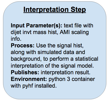
The final step of our VHbb analysis chain receives five inputs, four of which are for the MC scaling discussed in the last episode:

• normalized event-weighted h_mjj_kin_cal histogram
• sum of MC generator event weights
• predicted signal cross-section
• filter efficiency
• k-factor

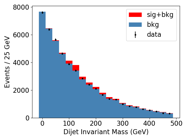
For our interpretation, mock background MC is generated from a falling exponential distribution and bin it with the same edges as the input signal histogram. A toy data histogram is then generated by randomly selecting the number of events in each bin from a Poisson distribution with mean λ equal to the amplitude of the equivalent background MC bin. We won’t go through the details of how this is coded during this tutorial - we provide the full image for this last step (but feel free to look through the gitlab repo that produces it later on if you’re curious). But if you’re keen to try doing the toy MC and data generation yourself, check out the next (optional) bonus exercise.

Here is a sample plot of the mock background, signal, and toy data produced by this step:

Exclusion vs. Discovery

You’ll notice that we haven’t incorporated the signal model into our toy data generation at all, so at present we don’t actually expect to find any evidence for our signal in the data. We could choose to add in some signal component and see at what point we can detect the signal, but for this tutorial we chose to keep the data consistent with background because (sadly…) given the lack of excesses we’ve seen so far with beyond-standard-model (BSM) searches at the LHC analysts doing these BSM searches are so far dealing with “exclusion” scenarios, where the data is found to be consistent with background, and the next step is to place an upper bound on the cross section, above which the analysis results exclude the existence of the signal to some degree of confidence (typically 95%). Please feel free to play around with the data generation and pyhf fit on your own later though and try out a discovery scenario!

Bonus Exercise!

Use your language of choice to write a program which:

a) Inputs the signal histogram we produced as a text file in the reformatting step

b) Generates 50000 MC background samples from an exponential distribution in dijet invariant mass with a decay constant of 150

c) Bins the generated MC background samples according to the binning of the signal histogram, and

d) Generates a toy data histogram, where the number of events in each bin is randomly generated from a Poisson distribution with central value λ equal to the amplitude of the MC background in the same bin.

Solution

For the solution implemented in python for this interpretation step, see lines 39-50 of run_fit.py

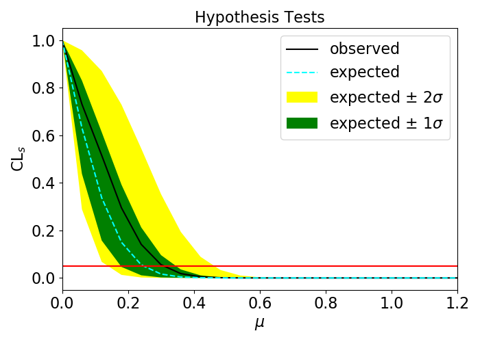
Finally, the signal, mock background, and toy data are passed through the pyhf interpretation to produce something called a μ-scan. The x axis is the hypothetical “signal strength” of a model where you hypothesize that the data is composed of:

data = μs + b

where s is the signal component and b is the background. The y-axis shows the CL_s, which is defined as the ratio of the p-value CL_s+b associated with comparing the data to the μs + b hypothesis to the p-value CL_b associated with the background-only hypothesis:

CL_s = CL_s+b / CL_b

The following figure shows a sample μ-scan produced by this step, where the observed CL_s variation is in this case within the expected bounds for a background-only hypothesis. Values of the signal strength μ above which the observed CL_s falls below the horizontal red line at CL_s=0.05 are excluded by the fit. Below these values, the statistics are too poor to confidently exclude these signal strengths.

Encoding the Interpretation Step

Please add the following to your steps.yml file to encode this final step:

interpretation_step:
  process:
    process_type: interpolated-script-cmd
    script: |
     python /code/run_fit.py \
            --inputfile {signal} \
            --xsection {xsection} \
            --sumofweights {sumweights} \
            --kfactor {kfactor} \
            --filterfactor {filterfactor} \
            --luminosity {luminosity} \
            --plotfile {plot_png} \
            --outputfile {fit_result}
  environment:
    environment_type: docker-encapsulated
    image: gitlab-registry.cern.ch/usatlas-computing-bootcamp/pyhf-fit
    imagetag: master
  publisher:
    publisher_type: interpolated-pub
    publish:
      inference_result: '{fit_result}'
      visualization: '{plot_png}'

and the corresponding workflow step to your workflow.yml:

- name: interpretation_step
  dependencies: [reformatting_step]
  scheduler:
    scheduler_type: singlestep-stage
    parameters:
      signal: {step: reformatting_step, output: hist_txt}
      xsection: {step: init, output: xsection}
      sumweights: {step: init, output: sumweights}
      kfactor: {step: init, output: kfactor}
      filterfactor: {step: init, output: filterfactor}
      luminosity: {step: init, output: luminosity}
      fit_result: '{workdir}/limit.png'
      plot_png: '{workdir}/hists.png'
    step: {$ref: steps.yml#/interpretation_step}

This step can be tested with the following packtivity_run command which incorporates all the scaling factors we’ve obtained:

packtivity-run -p signal="'{workdir}/workdir/reformatting_step/selected.txt'" -p xsection=44.837 -p sumweights=6813.025800 -p kfactor=1.
0 -p filterfactor=1.0 -p luminosity=140.1 -p plot_png="'{workdir}/hists.png'" -p fit_result="'{workdir}/limit.png'" steps.yml#/interpretation_step

With so many input parameters at this point, it gets a bit cumbersome to keep listing them on the command line - yadage has a solution for this! Create a new file called inputs.yml at the top level of your workflow directory, and fill it with the following:

signal_daod: recast_daod.root
xsection: 44.837
sumweights: 6813.025800
kfactor: 1.0
filterfactor: 1.0
luminosity: 140.1

The full yadage-run command can now be run as follows, with an optional third argument giving the name of the file with the input parameters:

yadage-run workdir workflow.yml inputs.yml -d initdir=$PWD/inputdata

Key Points

• The interpretation produces a μ-scan, which essentially represents a p-value as a function of the hypothesized signal strength μ.

• Our μ-scan result is consistent with the null background-only hypothesis.

• We haven’t delved into much detail on exactly how the pyhf code does its thing, but just knowing what it produces and how it’s executed is enough to encode the interpretation step with yadage.