Introducing Workflows

Overview

Teaching: 30 min
Exercises: 10 min

Questions

• What is the ultimate physics goal in interpreting our analysis of the VHbb signal model?

• What is the goal of RECAST in the context of interpreting our analysis?

• How does yadage help us preserve our analysis workflow for re-interpretation?

Objectives

• Understand the concept (but not necessarily the details!) of combining our signal model with data and SM background to interpret our analysis as a search for new physics.

• Get a high-level overview of how yadage can help you preserve your analysis for re-interpretation.

Introduction

Interpreting our Analysis

What do we want?

So far in our VHbb analysis, we’ve taken a Monte Carlo simulated signal DAOD, looped through this MC data event-by-event, applied some kinematic selections, and output the data to a histogram of the dijet invariant mass. But what we really want to do in the end is compare our simulated signal sample with data from the ATLAS detector to determine whether we can see our signal in the data, and if so, to what extent.

What would we do in a “real” analysis?

In a real analysis, a proper comparison with the data would require accounting for all the events from SM background processes that make it through our selection, and adding these events to our histograms. We could then perform a fit to determine whether the observed data is best explained by the SM background alone, or by some combination of the background and signal.

What are we actually going to do?

However, the time it would take us to properly account for all the SM backgrounds would probably take away from the main purpose of this “docker in ATLAS” tutorial. So we’ll instead assume that our SM background distribution can be modeled analytically by some smoothly decaying exponential in the dijet invariant mass, and move along (keeping in mind that this would in no way fly in a real analysis!). We’ll also provide some toy data for the interpretation. The fit will be done using a python fitting framework called pyhf.

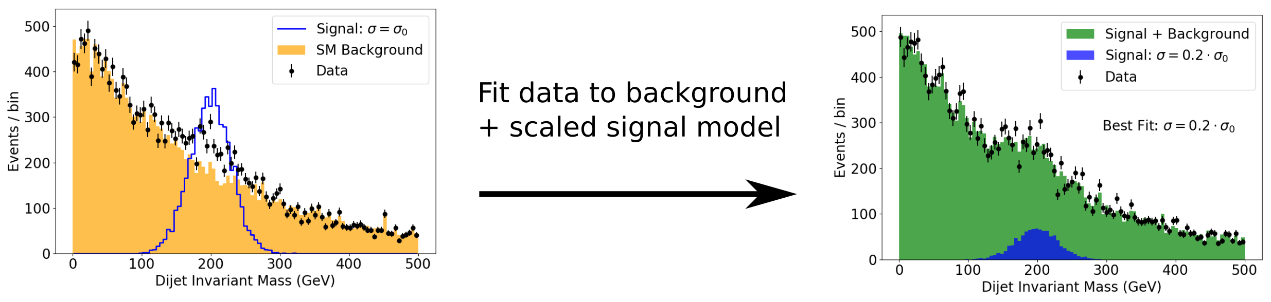
This approach is illustrated in the following doodle, where some data is fit with the background plus signal, with the signal amplitude (linearly proportional to the cross section) allowed to vary. The fit shows that the data is best represented with a signal component, where the signal cross section is 1/5th of its simulated value. Note that the signal in this doodle is not meant to represent our particular VHbb signal - it’s just drawn from a Gaussian distribution for illustration.

Analysis Preservation and Re-interpretation

Workflow preservation/automation

Thanks to gitlab and docker, we’ve now successfully preserved our analysis code and the environment in which we run it. The final piece of RECAST analysis preservation is to preserve our analysis workflow for interpreting the signal as described above, and automate the process of passing an arbitrary signal model through the workflow to re-interpret the analysis in a new context.

Why do we need to get fancy?

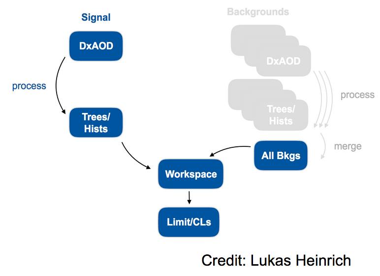
If it weren’t for the docker containers involved in RECAST, this could conceivably be accomplished with some environment variables and bash scripts that just list out each command that an analyst would type into the terminal while going through the analysis. But when we perform the analysis steps in docker containers, we need a way to codify what needs to happen in which container for each step, and how the output from one step feeds as the input for later steps. Lukas Heinrich has written a great tool called “yadage” to handle this situation. Before diving into the gory details of how to actually program with yadage, let’s start with a high-level overview of what it is and how it accomplishes the goal of preserving and re-interpreting our analysis.

Background preservation

Preserving background contributions to fit

In our sample analysis, we’re using an analytic falling exponential as our background, but a real ATLAS analysis will have many different sources of background, each obtained from its own set of DAODs, and involving its own set of systematics that will affect the fit result. Since these background contributions won’t change when the analysis is re-interpreted with a new model, it’s in general important to preserve the contribution of these backgrounds to the final analysis results in the analysis code so that one only needs to run the signal DAOD through the analysis chain when the analysis is re-interpreted with RECAST.

What RECAST doesn’t do

Another important point to keep in mind is that RECAST does not on its own document the exact version of Athena code that was originally used to produce your background and signal DAODs. Your code may not necessarily be compatible with DAODs produced with future releases of the ATLAS derivation framework. Therefore, it would be good document somewhere in your gitlab repo exactly which ATLASDerivation cache and p-tags were used to produce the DAODs used in your analysis (this could just be, eg. a list of all the dataset names used) so other analysts know to produce new signals for RECAST with this same version. See the DerivationProductionTeam page for more information about derivation production and organzation.

Yadage

Yadage is both:

• a syntax for describing workflows made up of containerized steps, and
• an execution engine for actually running these workflows.

We’ll get into the syntax part of yadage in the upcoming intermezzo lesson, during which you’ll get to practice writing a basic helloworld workflow in yadage. But before venturing too far into the forest of syntax, let’s first fly overhead and see where this is all going.

In the yadage approach, the workflow is divided into distinct steps, called packaged activities - or “packtivities” - each of which will run inside a docker container. The steps get linked into a workflow by specifying how the output from each such packtivity step feeds in as the input for subsequent steps (this flow of dependencies is not necessarily linear). The yadage workflow engine optimizes the execution of the workflow.

More reading on Yadage

Nice introductory yadage tutorial: https://yadage.github.io/tutorial/

Yadage and Packtivity – analysis preservation using parametrized workflows (paper on arXiv with lots of great background info)

Steps

Each step in the workflow is fully described by:

• Publisher descriptions: The input data that the step receives from previous step(s) - or from the user if it’s the first step in the workflow - and the output that it sends - i.e. “publishes” - to the next step.
• Process description: Instructions - typically a bash command or script - for transforming the input data into output to be fed into the next step, or the final result if it’s the last step in the workflow
• Environment description: The environment in which the instructions need to be executed. This is specified by the image used to start the container in which the step will run.

and these three components are codified with dedicated yadage syntax, as we’ll see in the upcoming “Yadage Helloworld” intermezzo.

VHbb RECAST Steps

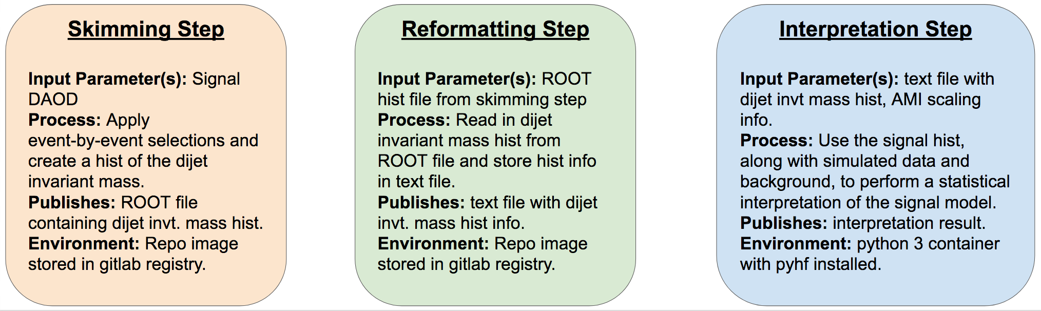
The three steps involved in interpreting our VHbb analysis are as follows:

• Skimming Step: This is the step that we’re already familiar with, where we take in the signal DAOD, loop through it event-by-event, apply some selections, and output a histogram of the dijet invariant mass variable that we’ll want to fit our model to the data. This step will take place in the custom AnalysisBase container we recently created for our analysis repo.
• Reformatting Step: The pyhf statistical interpretation framework that we’ll use for re-interpretation is written in pure python and runs outside of ROOT, so we can simplify the fitting step somewhat by reformatting the histogram that we wrote to a ROOT file in the previous skimming step into a text file that is readable in pure python, and outputting this text file to the interpretation step.
• Interpretation Step: Here, we use pyhf to do our statistical analysis of the signal, background, and data to determine whether we can detect our signal model in the data. We need some extra pieces of information to scale the signal appropriately, which we can get from the AMI database (this will be discussed further soon).

These steps are summarized in the following illustration:

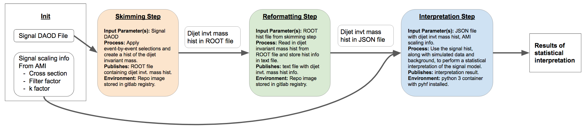
Workflow

The workflow description specifies how all the steps “fit together”. It accomplishes this by specifying exactly where all the data to be input to each step comes from - whether it be user-provided (i.e. “init” data) or output from a previous step - and how each step will be executed.

So here is an idea of what our workflow should look like:

Exercise (10 min)

Part 1

Giordon has already shown you how to make your code more flexible by making the path to the input file and the number of events to loop over optional input arguments to the AnalysisPayload executable. It would also be good for clarity (and in fact necessary if we wanted to start considering different background samples) to be able to specify the name of the ROOT file containing the output histograms depending on the input DAOD. But at present, the filename and path to the output ROOT file is hard-coded into the AnalysisPayload.cxx code.

So, with an eye on re-interpretation, update the AnalysisPayload.cxx in your gitlab repo so it can read in both:

• the path to the input DAOD, and
• the path to the output ROOT file that will contain the histograms created by AnalysisPayload.cxx

such that the AnalysisPayload executable can be executed as follows:

AnalysisPayload /path/to/input/DAOD.root.1 /path/to/output/ROOT/file.root number_of_events_to_loop_over

Part 2

Now, update the run stage in your .gitlab-ci.yml file so that the AnalysisPayload executable writes the output file to ci_outputFile.root and, again, loops over 1000 events.

Part 3

If you haven’t already, reduce the printout frequency in AnalysisPayload.cxx, since this is by far its rate-limiting factor:

To do this, add if(i%10000==0) in front of the two std::cout() printouts in the event loop.

Part 4

While we’re at it, we’ll also need to make the binning a bit coarser for when we output the histogram to the pyhf fitting step, since the pyhf fitter takes a lot longer to run with many bins without necessarily much/any gain in sensitivity. So let’s do that now. Update your AnalysisPayload.cxx so that it produces the h_mjj_* histograms with 20 rather than 100 bins.

Solution

Part 1

The updates should look something like:

Underneaath

if(argc >= 2) inputFilePath = argv[1];

add

TString outputFilePath = "myOutputFile.root";
if(argc >=3) outputFilePath = argv[2];

• TFile *fout = new TFile("myOutputFile.root","RECREATE"); –> TFile *fout = new TFile(outputFilePath), "RECREATE");

Part 2

- AnalysisPayload root://eosuser.cern.ch//eos/user/g/gstark/public/DAOD_EXOT27.17882744._000026.pool.root.1 1000

on line 49 becomes

- AnalysisPayload root://eosuser.cern.ch//eos/user/g/gstark/public/DAOD_EXOT27.17882744._000026.pool.root.1 ci_outputFile.root 1000

Part 4

The code to create the new h_mjj histogram objects should be updated as follows:

TH1D *h_mjj_raw = new TH1D("h_mjj_raw","",100,0,500); –> TH1D *h_mjj_raw = new TH1D("h_mjj_raw","",20,0,500);

TH1D *h_mjj_kin = new TH1D("h_mjj_kin","",100,0,500); –> TH1D *h_mjj_kin = new TH1D("h_mjj_kin","",20,0,500);

TH1D *h_mjj_raw_cal = new TH1D("h_mjj_raw_cal","",100,0,500); –> TH1D *h_mjj_raw_cal = new TH1D("h_mjj_raw_cal","",20,0,500);

TH1D *h_mjj_kin_cal = new TH1D("h_mjj_kin_cal","",100,0,500); –> TH1D *h_mjj_kin_cal = new TH1D("h_mjj_kin_cal","",20,0,500);

Once you’re happy with your updates to AnalysisPayload.cxx, you can commit and push them to your gitlab repo.

Hints

• You can test your updates by volume-mounting your repo directory and DAOD to the atlas/analysisbase:21.2.85-centos7:

cd /top/level/of/local/gitlab/repo
docker run --rm -it -v /path/to/DAOD:/Data/signal_daod.root -v $PWD:/Bootcamp atlas/analysisbase:21.2.85-centos7 bash

• Part 1 should require changing three lines in AnalysisPayload.cxx (and adding one additional line). Part 2 should require changing four lines.

• The simplest way to implement command-line arguments in C/C++ is by passing the number argc of command line arguments and the list **argv of arguments to the main() function (see eg. this quick cplusplus.com tutorial).

Key Points

• Our end goal with the VHbb analysis is to perform a statistical comparison of our signal model with ATLAS data and SM backgrounds to determine whether we can see evidence of the signal in the data.

• The goal of RECAST is to preserve and automate the procedure of re-interpreting our analysis with a new signal model.

• Yadage helps you preserve each step of passing an arbitrary signal model through our analysis chain as a containerized process, and combine these steps into an automated workflow.

• Try to avoid hard-coding anything to do with the signal model while developing your analysis, since this info will change when it’s re-interpreted. Better yet, maintain your RECAST framework as you develop your analysis so you don’t even have to think about it!